Soma Cube – Aswin van Woudenberg

The Soma cube is the brainchild of Danish mathematician, inventor, designer, writer and poet Piet Hein. The puzzle consists of seven pieces and the goal is to assemble these pieces into a 3x3x3 cube or other shapes.

Piet Hein came up with this puzzle during a lecture on quantum physics by Werner Heisenberg. Instead of paying attention to the renowned theoretical physicist, Piet prefered idling away his time by thinking up frivolous brainteasers. Such a waste, not to mention rude! What’s even worse is that people seemed to actually enjoy his puzzle. This meant that Piet Hein’s invention wasn’t just a time-waster for him but for everyone who got hooked on it.

Initially, the Soma cube was mostly known in Scandinavian countries, but things took a dark turn when Martin Gardner featured it in his Mathematical Games column in Scientific American in September 1958. Suddenly, the whole world got introduced to this time-waster.

As a self-proclaimed restorer of productivity, I hate to see people trifle away their lives trying to solve these inane puzzles. For this reason I’ve created a Soma solver in Python so people can go back to spending time on more fruitful pursuits.

Read on to learn how I did this.

The Soma puzzle pieces

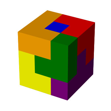
Each of the seven pieces has a different shape. I’ve given each shape a different color to ease visualizing solutions later on.

As mentioned above, the objective is to assemble these pieces into various shapes, like a cube.

Importing libraries

Let’s start by importing some libraries. We’ll use matplotlib to visualize solutions in 3D.

import numpy as np
import matplotlib.pyplot as plt
import matplotlib.animation as animation
import ipywidgets as widgets

from IPython.display import HTML
from math import ceil

Representing the pieces

We’ll represent each piece as a list of coordinates in 3D space. Each tuple is an (x, y, z) coordinate.

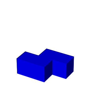
z = [(0,0,0),(1,0,0),(1,1,0),(2,1,0)] # blue piece
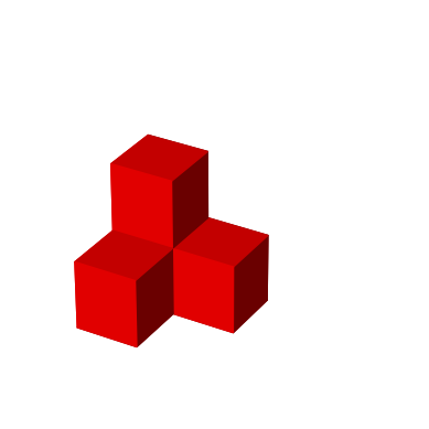
p = [(0,0,0),(0,1,0),(0,1,1),(1,1,0)] # red piece
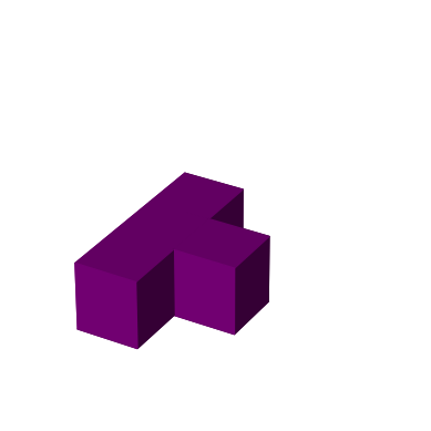
t = [(0,0,0),(0,1,0),(1,1,0),(0,2,0)] # purple piece
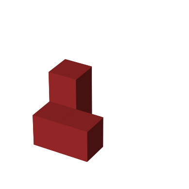
b = [(0,0,0),(1,0,0),(0,1,0),(0,1,1)] # brown piece
a = [(0,0,0),(0,0,1),(0,1,0),(1,1,0)] # yellow piece
l = [(0,0,0),(1,0,0),(2,0,0),(0,1,0)] # orange piece
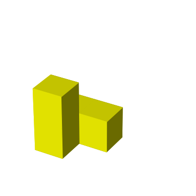
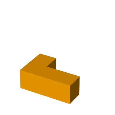
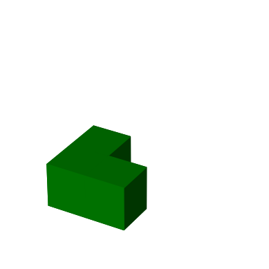
v = [(0,0,0),(1,0,0),(0,1,0)] # green piece

The letters z, t, p, b, a, l, and v look (with some imagination) like the pieces.

Let’s put all pieces and colors in a list so we can access them by index.

pieces = [z, p, t, b, a, l, v]
colors = ["blue", "red", "purple", "brown", "yellow", "orange", "green"]

Visualizing the pieces and solution

Before writing the solver, let’s consider how we can create a 3D visualization of the Soma cube. I’ve chosen to use Matplotlib for its 3D rendering capabilities.

Matplotlib can draw voxels (3D pixels) which we can use to visualize a single piece, multiple pieces, or even the full solution in 3D. The following function takes a 3D numpy array that represents the voxels and plots them.

def plot_solution(colors, ax=None):
    if not ax:
        fig = plt.figure()

        # axis with 3D projection
        ax = fig.add_subplot(projection='3d')
        
    ax.set_aspect('equal')
    ax.set_axis_off()

    # draw each voxel with a color (each voxel unequal to None)
    voxels = (colors != None)

    ax.voxels(voxels, facecolors=colors, edgecolors=colors)

To use this function we need to call it with a 3D numpy array that represents each voxel.

voxels = np.empty((3,3,3), dtype='object')

Each element in this array is initialized to None.

voxels

array([[[None, None, None],
        [None, None, None],
        [None, None, None]],

       [[None, None, None],
        [None, None, None],
        [None, None, None]],

       [[None, None, None],
        [None, None, None],
        [None, None, None]]], dtype=object)

Let’s set each element of voxels to a color and call plot_solution. We can set elements seperately, like this:

voxels[0][0][0] = 'yellow'
voxels[1][0][0] = 'yellow'
voxels[0][0][1] = 'yellow'
voxels[0][1][1] = 'yellow'

Or we can set all elements at once.

voxels = np.array([
    [['yellow', 'yellow', 'orange'],
     ['brown',  'yellow', 'orange'],
     ['brown',  'brown',  'orange']],
    [['yellow', 'green',  'orange'],
     ['brown',  'blue',   'blue'],
     ['blue',   'blue',   'red']],
    [['purple', 'green',  'green'],
     ['purple', 'purple', 'red'],
     ['purple', 'red',    'red']]
])

plot_solution(voxels)
plt.show()

This is the same solution as shown above and one of the 240 possible unique ways of packing the seven Soma pieces into a 3x3x3 cube.

Let’s see how we can visualize a single piece.

def plot_piece(piece, color, ax=None):
    max_dim = np.max([np.max(piece) + 1, 3])
    voxels = np.empty((max_dim, max_dim, max_dim), dtype='object')
    for x, y, z in piece:
        voxels[x][y][z] = color
    plot_solution(voxels, ax)

plot_piece(z, "blue")
plt.show()

Animating a solution

In the solution above it was impossible to tell how some pieces were positioned. The following function animates the assembly of a solution by adding pieces one by one.

def animate_solution(colors):
    w, d, h = colors.shape
    
    show_order = []
    for a in range(1,max(w, d, h)+1):
        for z in range(min(a,h)):
            for x in range(min(a,w)):
                for y in range(d-1,d-1-min(a,d),-1):
                    color = colors[x][y][z]
                    if not (color is None or color in show_order):
                        show_order.append(color)
    
    fig = plt.figure()
    
    ax = fig.add_subplot(projection='3d')
    
    def update(frame):
        ax.clear()
        ax.set_aspect('equal')
        ax.set_axis_off()
        
        voxels = np.in1d(colors, show_order[:frame+1]).reshape(colors.shape)

        ax.voxels(voxels, facecolors=colors, edgecolors=colors)

    plt.close()

    anim = animation.FuncAnimation(fig, update, frames=len(show_order), interval=1000)
    
    return anim

anim = animate_solution(voxels)
HTML(anim.to_jshtml(default_mode='once'))

Now it’s much clearer how a solution is constructed.

Rotating pieces

We will implement the solver using a simple recursive backtracking algorithm. The solver will try to fit the pieces in their various orientations. For this reason, we define some helper functions to rotate a piece around an axis. I also defined an identity function that just returns the input as is. Its use will become clear later.

rotate_x = lambda cubelets: [(x, z, -y) for (x, y, z) in cubelets]
rotate_y = lambda cubelets: [(z, y, -x) for (x, y, z) in cubelets]
rotate_z = lambda cubelets: [(-y, x, z) for (x, y, z) in cubelets]
identity = lambda cubelets: cubelets

For instance, to rotate piece z around the x-axis we can make use of rotate_x.

rotate_x(z)

[(0, 0, 0), (1, 0, 0), (1, 0, -1), (2, 0, -1)]

We can see that rotating a piece may make some coordinates negative. The following function translates a piece so that all x, y, z coordinates are minimal but positive.

def translate(piece):
    d_x, d_y, d_z = np.min(np.array(piece), axis=0) * -1
    return [(x + d_x, y + d_y, z + d_z) for (x, y, z) in piece]

Now we can do the same rotation as above but end up with coordinates that are all positive.

translate(rotate_x(z))

[(0, 0, 1), (1, 0, 1), (1, 0, 0), (2, 0, 0)]

We will use this translate function when we display individual pieces.

Generating all orientations for each piece

Using the functions defined above we can generate all orientations for each piece. Several transformations are performed one after another. The identity function just returns the original orientation.

def generate_rotations(piece):
    orientations = []
    for f_a in [identity, rotate_x,  rotate_y, rotate_z]:
        for f_b in [identity, rotate_x,  rotate_y, rotate_z]:
            for f_c in [identity, rotate_x,  rotate_y, rotate_z]:
                for f_d in [identity, rotate_x,  rotate_y, rotate_z]:
                    for f_e in [identity, rotate_x,  rotate_y, rotate_z]:
                        rot_piece = sorted(f_a(f_b(f_c(f_d(f_e(piece))))))
                        min_x, min_y, min_z = rot_piece[0]
                        trans_rot_piece = [(x - min_x, y - min_y, z - min_z) for x, y, z in rot_piece]
                        if trans_rot_piece not in orientations:
                            orientations.append(trans_rot_piece)
                        
    return orientations

We can call this function for one piece.

generate_rotations(z)

[[(0, 0, 0), (1, 0, 0), (1, 1, 0), (2, 1, 0)],
 [(0, 0, 0), (1, 0, -1), (1, 0, 0), (2, 0, -1)],
 [(0, 0, 0), (0, 0, 1), (0, 1, -1), (0, 1, 0)],
 [(0, 0, 0), (0, 1, 0), (1, -1, 0), (1, 0, 0)],
 [(0, 0, 0), (1, -1, 0), (1, 0, 0), (2, -1, 0)],
 [(0, 0, 0), (0, 1, 0), (0, 1, 1), (0, 2, 1)],
 [(0, 0, 0), (0, 0, 1), (1, 0, 1), (1, 0, 2)],
 [(0, 0, 0), (0, 1, -1), (0, 1, 0), (0, 2, -1)],
 [(0, 0, 0), (1, 0, 0), (1, 0, 1), (2, 0, 1)],
 [(0, 0, 0), (0, 1, 0), (1, 1, 0), (1, 2, 0)],
 [(0, 0, 0), (0, 0, 1), (0, 1, 1), (0, 1, 2)],
 [(0, 0, 0), (0, 0, 1), (1, 0, -1), (1, 0, 0)]]

Or we can apply this function to every piece in the pieces list we defined above.

orientations = list(map(generate_rotations, pieces))

We can display all orientations for each piece. Note how we apply translate to make sure all coordinates end up in the positive quadrant.

cols = 8
total_number_of_orientations = sum(list(map(len,orientations)))
rows = ceil(total_number_of_orientations / cols)
fig, axs = plt.subplots(rows, cols, figsize=(cols*3,rows*3), 
    subplot_kw= { 'projection':'3d' }, gridspec_kw = {'wspace':0.0, 'hspace':0.0})

fig.subplots_adjust(top=0.96)
fig.suptitle(f"Orientations", fontsize=16)

count = 0
for i in range(len(pieces)):
    for j in range(len(orientations[i])):
        plot_piece(translate(orientations[i][j]), colors[i], axs[count // cols, count % cols])
        count += 1

while count < cols * rows:
    axs[count // cols, count % cols].set_axis_off()
    count += 1

plt.show()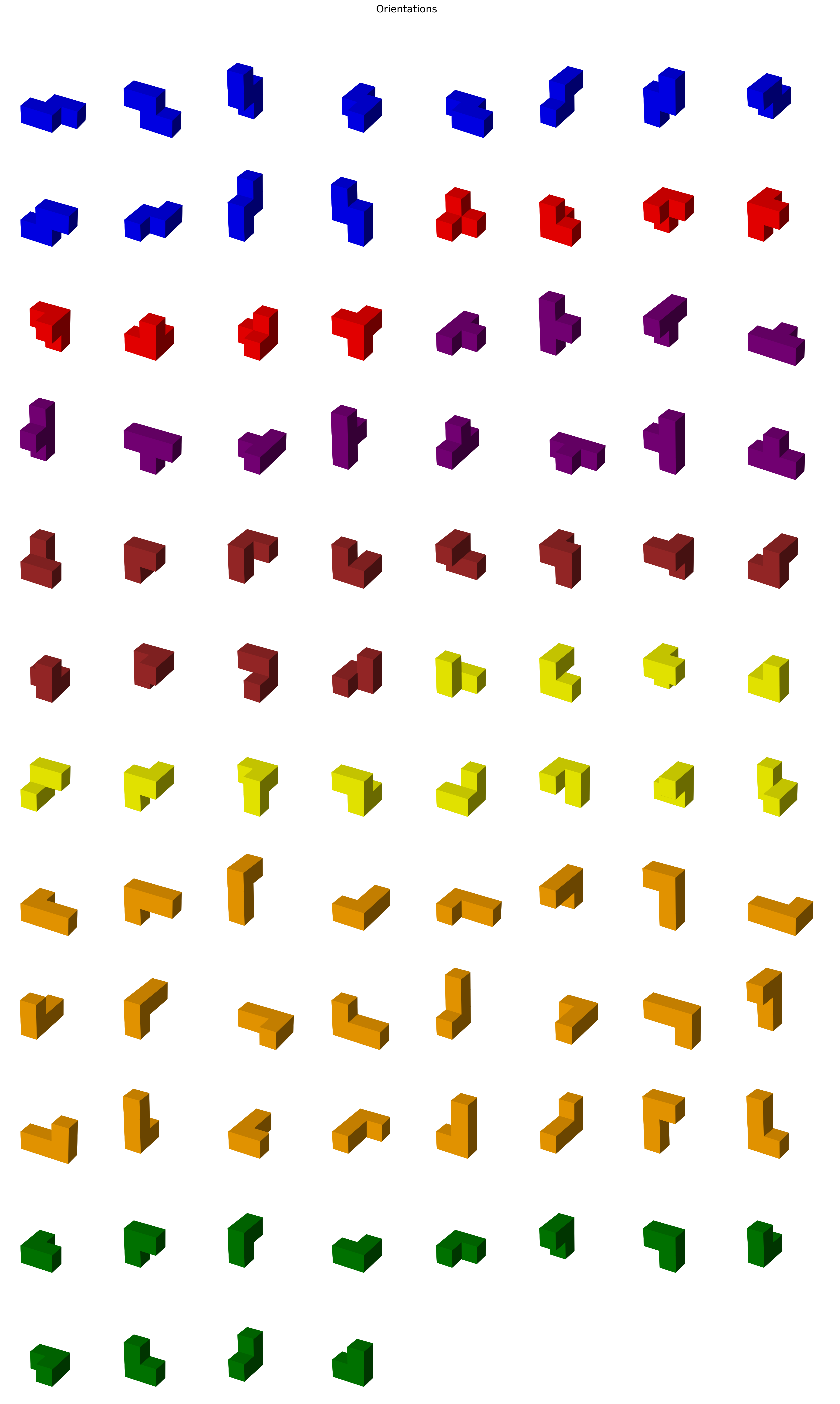

In the solver below, for each piece we’ll see which orientation fits where.

Writing the solver

We’re finally ready to work on the solver for the Soma cube. The solver will take in a list of coordinates (that make up the cube that we want to fill up with pieces) and recursively search for a solution.

We can generate this list of coordinates using a simple list comprehension.

cube_coordinates = [(x, y, z) for x in range(3) for y in range(3) for z in range(3)]

cube_coordinates

[(0, 0, 0),
 (0, 0, 1),
 (0, 0, 2),
 (0, 1, 0),
 (0, 1, 1),
 (0, 1, 2),
 (0, 2, 0),
 (0, 2, 1),
 (0, 2, 2),
 (1, 0, 0),
 (1, 0, 1),
 (1, 0, 2),
 (1, 1, 0),
 (1, 1, 1),
 (1, 1, 2),
 (1, 2, 0),
 (1, 2, 1),
 (1, 2, 2),
 (2, 0, 0),
 (2, 0, 1),
 (2, 0, 2),
 (2, 1, 0),
 (2, 1, 1),
 (2, 1, 2),
 (2, 2, 0),
 (2, 2, 1),
 (2, 2, 2)]

The solver will yield the same list but each tuple will have an extra element indicating the color that coordinate will get after all pieces have been placed.

We’ll use a list of booleans to keep track of which pieces have been placed.

pieces_used = [False] * 7

def solve_soma_(solution, i):
    if i == 27:
        yield solution
    else:
        x, y, z, _ = solution[i]
        for piece in range(7):
            if not pieces_used[piece]:
                for orientation in orientations[piece]:
                    empty_coords = [(x + d_x, y + d_y, z + d_z, None) for (d_x, d_y, d_z) in orientation]
                    if all([tup in solution for tup in empty_coords]):
                        # placing piece: replace None with color
                        pieces_used[piece] = True
                        filled_coords = [(x + d_x, y + d_y, z + d_z, colors[piece]) for (d_x, d_y, d_z) in orientation]
                        new_solution = sorted([tup for tup in solution if tup not in empty_coords] + filled_coords)
                        
                        # find next empty coordinate
                        j = i
                        while j < 27 and new_solution[j][3]:
                            j += 1
                            
                        # continue search
                        yield from solve_soma_(new_solution, j)
                        pieces_used[piece] = False

def solve_soma(coordinates):
    global pieces_used
    pieces_used = [False] * 7
    
    solution = sorted([(x, y, z, None) for x, y, z in coordinates])
    yield from solve_soma_(solution, 0)

You call the solve_soma function with a list of coordinates representing the space that will be packed with Soma pieces. The actual algorithm is implemented in solve_soma_. The algorithm does the following:

It checks if all coordinates are filled. If so, it yields the solution.
For each possible orientation of a piece, it checks if it can be placed from the current coordinate without overlapping with filled coordinates that are already in the solution.
If a valid placement is found, it recursively explores how to fill from the next empty coordinate.
After exploring a piece and its orientation, it tries other possibilities.

Different solutions may be duplicates of each other in the sense that one solution is a rotation of another.

Finding and displaying a solution

The solver is a generator function that yields all solutions one by one. Let’s start by just displaying the first solution it finds.

The following function finds the first solution given a list of coordinates to fill and plots this solution.

def solve_and_plot_first_solution(coordinates, ax=None):
    # instantiate generator
    gen = solve_soma(coordinates)

    # find first solution
    solution = next(gen)

    # find voxel space size
    max_dim = np.max(coordinates) + 1

    # fill 3D voxel array and plot it
    voxels = np.empty((max_dim, max_dim, max_dim), dtype='object')
    for x, y, z, color in solution:
        voxels[x][y][z] = color

    plot_solution(voxels, ax)

solve_and_plot_first_solution(cube_coordinates)
plt.show()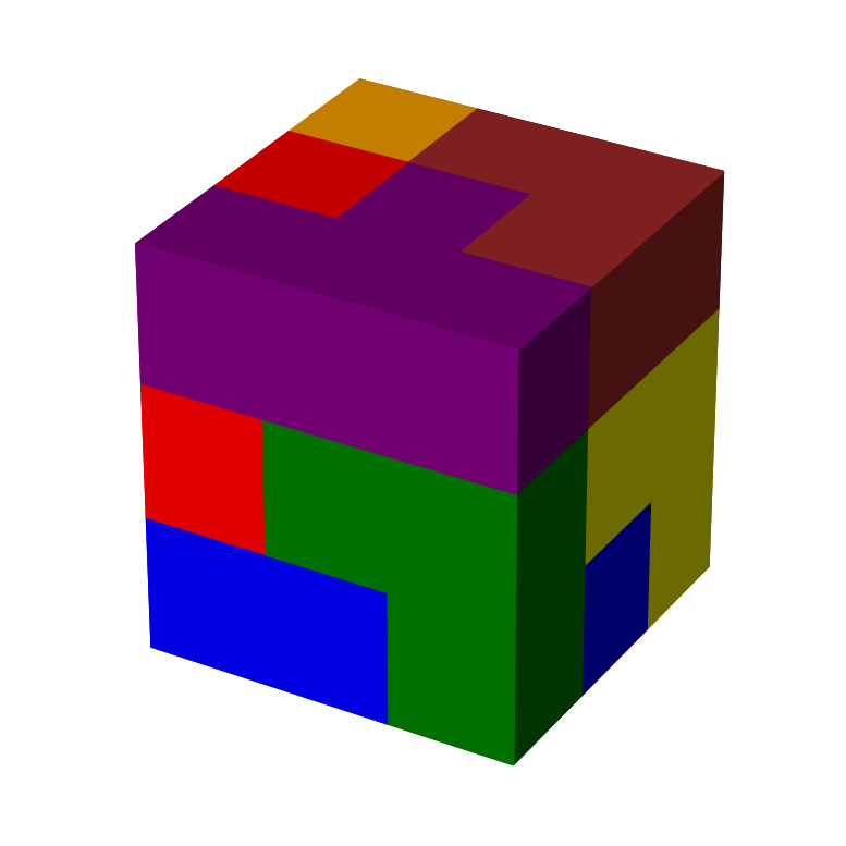

We’ll also define a function that finds the first solution and then animates it.

def solve_and_animate_first_solution(coordinates):
    # instantiate generator
    gen = solve_soma(coordinates)

    # find first solution
    solution = next(gen)

    # find voxel space size
    max_dim = np.max(coordinates) + 1

    # fill 3D voxel array and plot it
    voxels = np.empty((max_dim, max_dim, max_dim), dtype='object')
    for x, y, z, color in solution:
        voxels[x][y][z] = color

    anim = animate_solution(voxels)
    display(HTML(anim.to_jshtml(default_mode='once')))

solve_and_animate_first_solution(cube_coordinates)

Creating other figures

We called the solver with cube_coordinates that contains the coordinates that make up a cube. Instead of a cube, we can also pass a sorted list of coordinates that make up another shape.

Let’s look at some examples.

pyramid_coordinates = sorted(
    [(x, y, 0) for x in range(1, 4) for y in range(5)] + 
    [(x, y, 0) for x in [0, 4] for y in range(1, 4)] +
    [(2, y, 1) for y in range(1, 4)] + 
    [(1, 2, 1), (3, 2, 1), (2, 2, 2)]
)

turtle_coordinates = sorted(
    [(x, y, z) for x in range(1, 4) for y in range(1, 4) for z in range(2)] +
    [(4, 2, z) for z in range(3)] + 
    [(0, 2, 0), (1, 0, 0), (1, 4, 0), (3, 0, 0), (3, 4, 0), (5, 2, 2)]
)

tower_coordinates = sorted(
    [(x, y, z) for x in range(2) for y in range(2) for z in range(7) if (x, y, z) != (1, 0, 6)]
)

bear_coordinates = sorted(
    [(x, y, 0) for x in range(3) for y in range(2)] +
    [(x, 1, z) for x in range(3) for z in range(1, 6)] + 
    [(x, 0, z) for x in [0, 2] for z in [1, 3, 4]]
)

tunnel_coordinates = sorted(
    [(x, y, 0) for x in range(5) for y in range(3) if x != 2] +
    [(x, y, 1) for x in range(1, 4) for y in range(3) if x != 2] +
    [(x, y, 2) for x in range(1, 4) for y in range(3)]
)

tub_coordinates = sorted(
    [(x, y, 0) for x in range(5) for y in range(3)] +
    [(x, y, 1) for x in range(5) for y in range(3) if x in [0, 4] or y in [0, 2]]
)

airplane_coordinates = sorted(
    [(x, y, 0) for x in range(1, 6) for y in range(7) if x == 3 or y in [0, 1]] +
    [(x, y, 1) for x in range(7) for y in range(7) if y == 0 or (x == 3 and y != 5)]
)

bench_coordinates = sorted(
    [(x, y, z) for x in range(5) for y in range(2) for z in range(3) if y == 1 or x in [0, 4]] +
    [(x, 0, 1) for x in range(1, 4)] +
    [(x, 1, 3) for x in range(1, 4)]
)

duck_coordinates = sorted(
    [(x, y, z) for x in range(4) for y in range(3) for z in range(2)] +
    [(3, 1, 2), (3, 1, 3), (4, 1, 3)]
)

cascade_coordinates = sorted(
    [(x, y, z) for x in range(3) for y in range(3) for z in range(5) if (2-x) + y >= z]
)

chair_coordinates = sorted(
    [(x, y, z) for x in range(3) for y in range(3) for z in range(2)] +
    [(x, 2, z) for x in range(3) for z in range(2, 5)]
)

castle_coordinates = sorted(
    [(x, y, 0) for x in range(5) for y in range(5) if (x, y) not in [(0,2), (4,2)]] +
    [(0, 0, 1), (0, 4, 1), (4, 0, 1), (4, 4, 1)]
)

dog_coordinates = sorted(
    [(x, y, 0) for x in range(6) for y in range(3) if (x, y) not in [(3, 0), (3, 2), (5, 1)]] +
    [(x, y, 1) for x in range(5) for y in range(3) if x == 4 or y == 1] +
    [(x, 1, z) for x in range(3, 6) for z in range(2, 4) if (x, z) != (5, 3)]
)

cross_coordinates = sorted(
    [(x, y, z) for x in range(3) for y in range(3) for z in range(2)] +
    [(1, y, 2) for y in range(3)] +
    [(1, 1, z) for z in range(3, 7)] + 
    [(0, 1, 5), (2, 1, 5)]
)

elephant_coordinates = sorted(
    [(0, 0, 0), (3, 0, 0), (0, 2, 0), (3, 2, 0)] + 
    [(x, y, 1) for x in range(4) for y in range(3) if (x, y) != (3, 1)] +
    [(x, 1, z) for x in range(5) for z in range(2, 4) if (x, z) != (0, 3)] +
    [(4, 1, 1), (2, 0, 2), (2, 2, 2)]
)

stairs_coordinates = sorted(
    [(x, y, z) for y in range(3) for z in range(3) for x in range(4-z)]
)

snake_coordinates = sorted(
    [(x, y, z) for y in range(4) for z in range(2) for x in range(2*(3-y), (2*(3-y))+3)] +
    [(x, 0, z) for x in range(8, 10) for z in range(2, 4) if x == 8 or z == 3]
)

skyscraper_coordinates = sorted(
    [(x, y, 0) for x in range(3) for y in range(3)] +
    [(x, y, z) for x in range(2) for y in range(1, 3) for z in range(1, 5)] + 
    [(1, 1, 5), (1, 1, 6)]
)

wall_coordinates = sorted(
    [(x, x - 1, 0) for x in range(1, 6)] +
    [(x, x, z) for x in range(6) for z in range(2)] +
    [(x, x + 1, z) for x in range(5) for z in range(2)]
)

Let’s place these figures and their names into lists.

figure_names = ["Cube", "Pyramid", "Turtle", "Tower", "Bear", "Tunnel", "Tub", "Airplane", 
                "Bench", "Duck", "Cascade", "Chair", "Castle", "Dog", "Cross", "Elephant",
                "Stairs", "Snake", "Skyscraper", "Wall"
               ]
figure_coordinates = [
    cube_coordinates, pyramid_coordinates, turtle_coordinates, 
    tower_coordinates, bear_coordinates, tunnel_coordinates,
    tub_coordinates, airplane_coordinates, bench_coordinates,
    duck_coordinates, cascade_coordinates, chair_coordinates,
    castle_coordinates, dog_coordinates, cross_coordinates,
    elephant_coordinates, stairs_coordinates, snake_coordinates,
    skyscraper_coordinates, wall_coordinates
]

You can add more figures if you want. Just make sure that each list contains exactly 27 coordinates.

We can plot all figures as subplots.

cols = 5
number_of_figures = len(figure_coordinates)
rows = ceil(number_of_figures / cols)
fig, axs = plt.subplots(rows, cols, figsize=(cols*3,rows*3), 
    subplot_kw= { 'projection':'3d' }, gridspec_kw = {'wspace':0.5, 'hspace':0.0})

fig.suptitle(f"Figures", fontsize=16)

count = 0
for i in range(number_of_figures):
    solve_and_plot_first_solution(figure_coordinates[i], axs[count // cols, count % cols])
    axs[count // cols, count % cols].set_title(figure_names[i])
    count += 1

while count < cols * rows:
    axs[count // cols, count % cols].set_axis_off()
    count += 1

plt.show()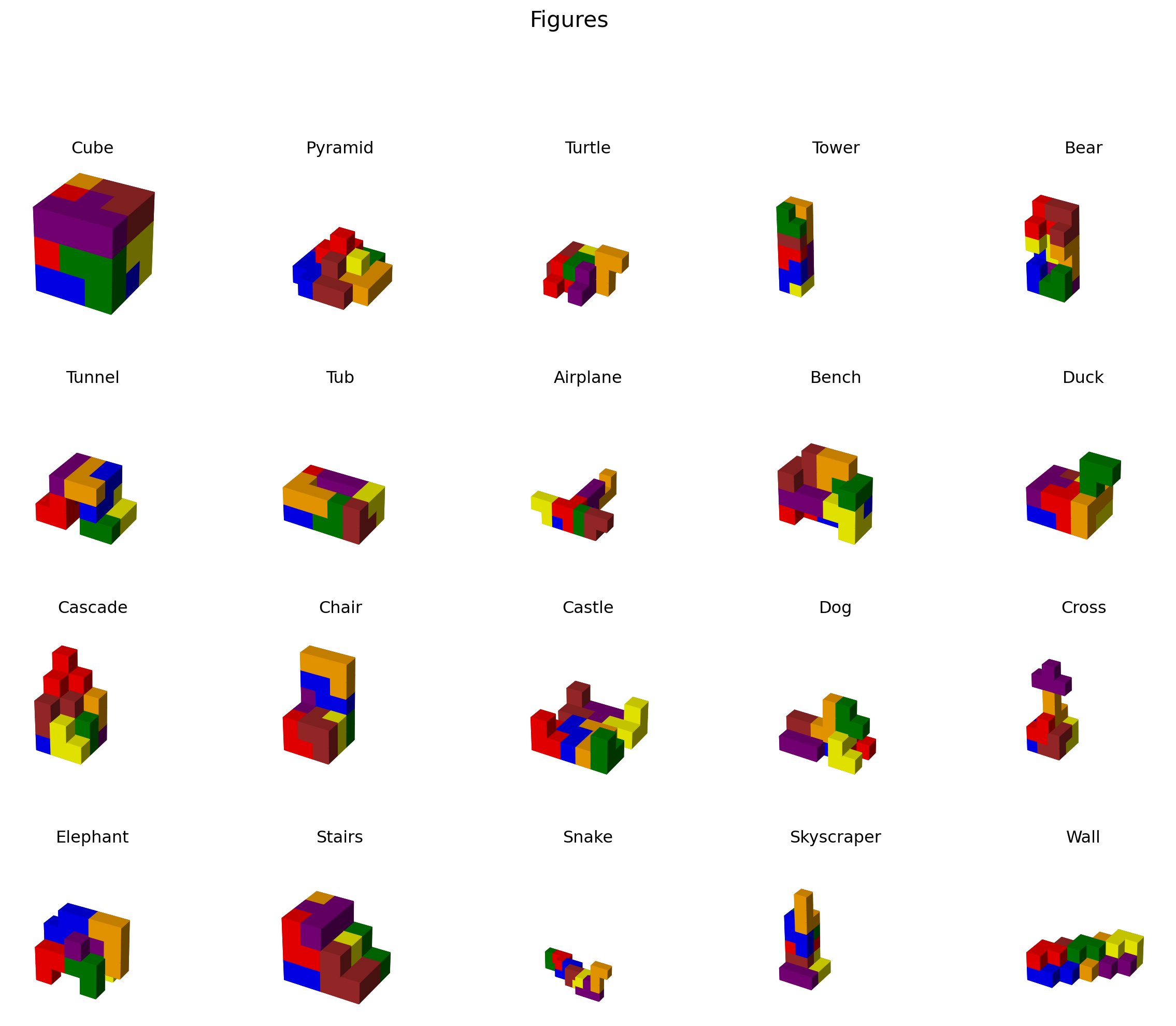

I have to admit that some figures are pretty cute.

Showing solutions one by one

Most figures can be assembled in more than one way. Using some widgets we can put together a simple GUI that lets us select a figure, solve it and iterate over the solutions.

We’ll use a dropdown menu, a button, an output widget, and a label widget. The solutions are shown as an animation we can step through.

figure_dropdown = widgets.Dropdown(options=zip(figure_names, figure_coordinates), value=cube_coordinates, description="Figure: ")
next_button = widgets.Button(description="Next")
hbox = widgets.HBox([figure_dropdown, next_button])
output = widgets.Output()
label = widgets.Label()

display(hbox, output, label)

To keep track of which solution to show next, we declare the following global variables:

gen = None
solution = None

The gen is a generator object that generates solutions for a given figure using the solve_soma function. The solution variable stores the next solution to be displayed. It is updated each time the “Next” button is clicked to display the next solution.

def figure_dropdown_change(change):
    global gen
    global solution
    
    if change['type'] == 'change' and change['name'] == 'value':
        value = change['new']
        next_button.layout.display = 'none'
        
        output.clear_output()
        
        gen = solve_soma(value)
        try:
            solution = next(gen)            
            with output:
                # find voxel space size
                max_dim = np.max(value) + 1

                # fill 3D voxel array and plot it
                voxels = np.empty((max_dim, max_dim, max_dim), dtype='object')
                for x, y, z, color in solution:
                    voxels[x][y][z] = color

                anim = animate_solution(voxels)
                display(HTML(anim.to_jshtml(default_mode='once')))
        except StopIteration:
            label.value = "No solutions found."
            return

        try:
            solution = next(gen).copy()
            label.value = ""
            next_button.layout.display = 'inline-block'
        except StopIteration:
            label.value = ""

figure_dropdown.observe(figure_dropdown_change)

The figure_dropdown_change function handles changes to the figure dropdown menu. It clears the output widget, displays the first solution, and stores the next solution in the solution variable (if any).

def on_next_button_clicked(b):
    global gen
    global solution
    
    output.clear_output(wait=True)
    with output:
        # find voxel space size
        max_dim = np.max(figure_dropdown.value) + 1

        # fill 3D voxel array and plot it
        voxels = np.empty((max_dim, max_dim, max_dim), dtype='object')
        for x, y, z, color in solution:
            voxels[x][y][z] = color

        anim = animate_solution(voxels)
        display(HTML(anim.to_jshtml(default_mode='once')))
    
    try:
        solution = next(gen)
    except StopIteration:
        label.value = ""
        next_button.layout.display = 'none'

next_button.on_click(on_next_button_clicked)

figure_dropdown_change({'type': 'change', 'name': 'value', 'new': figure_dropdown.value})

The on_next_button_clicked function handles clicks on the “Next” button by clearing the output widget, displaying the current solution, and generating the next solution.

Solving your own Soma puzzles

There you have it! No more wasting time on solving Soma puzzles. If you want to experiment with an interactive version of the solver, you can check out on of the following links:

Now go do something useful!